Turn you raw signals into insights with MDCplus
Try it yourself Get guided demo29 June 2026
From Raw Signals to Useful Metrics
How raw machine signals actually become dashboard metrics: state detection, aggregation, and calculation logic, with a worked example and common pitfalls
How can I use the data from HMI?
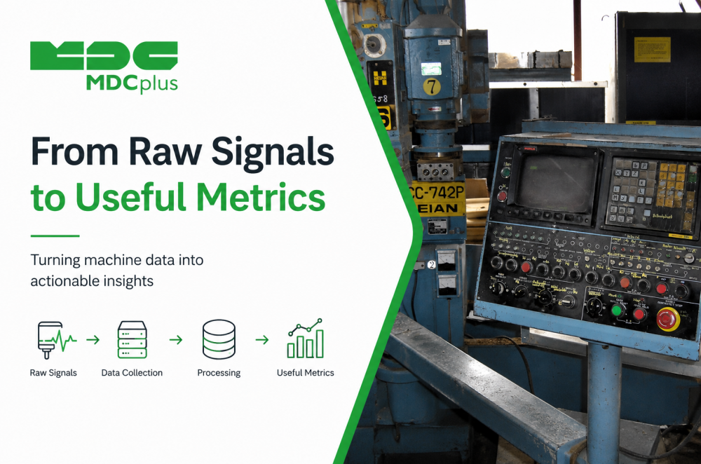
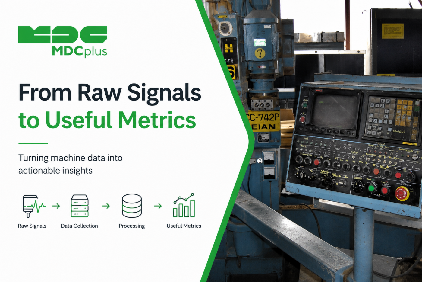
A spindle load reading of 42% doesn't mean anything on its own. Neither does a timestamp, a program number, or a single alarm code. Metrics like uptime, OEE, or average cycle time only exist because raw signals go through a series of transformations first — and that transformation logic is where a lot of monitoring projects quietly succeed or fail. This article walks through how raw data actually becomes something a plant manager can act on.
Contents:
- The gap between a signal and a metric
- The transformation pipeline
- Common types of transformations
- A worked example: from spindle state to Availability
- Where this logic should live
- Common pitfalls
- Frequently asked questions
- Conclusion
The gap between a signal and a metric
A raw signal is a single reading at a single moment: this axis is at this position, this alarm code is active, this program is running. A metric is a derived, aggregated, and interpreted number: this machine ran 82% of its scheduled time yesterday. Getting from one to the other involves several distinct steps — deciding what a signal actually means, tracking it over time, combining it with other signals, and applying a formula. Skipping over this gap and assuming metrics simply "appear" once data starts flowing is one of the more common misunderstandings in monitoring projects.
The transformation pipeline
- Interpretation. A raw value gets assigned meaning — a specific alarm code is classified as a specific downtime reason, a spindle load above a threshold is interpreted as "cutting."
- State detection. Individual signals are combined into a defined machine state — running, idle, in alarm, changeover — often requiring several raw inputs together rather than one signal alone.
- Time tracking. States are tracked over time, converting point-in-time readings into durations: how long was the machine in each state during a given period.
- Aggregation. Durations and counts are summed or averaged over a chosen period — a shift, a day, a job — to produce the numbers that actually get reported.
- Calculation. Final formulas (like Availability × Performance × Quality for OEE) combine aggregated values into the metrics people actually look at.
Common types of transformations
| Transformation type | Example |
|---|---|
| Thresholding | Spindle load above X% counts as "cutting," below counts as "idle" |
| Debouncing / filtering | Ignoring state changes shorter than a defined minimum duration to avoid false starts/stops from noisy signals |
| Counting | Incrementing a part counter each time a defined cycle-complete signal occurs |
| Duration summing | Adding up total minutes in "running" state across a shift |
| Ratio calculation | Dividing actual output by ideal output to get a Performance percentage |
| Classification | Mapping a specific alarm code to a human-readable downtime category |
A worked example: from spindle state to Availability
- Step 1 — raw signal: the connection layer reports spindle load as a numeric value every second: 0%, 0%, 45%, 48%, 44%, 0%, 0%...
- Step 2 — interpretation: a threshold rule defines spindle load above 5% as "cutting" and below as "not cutting."
- Step 3 — debouncing: a minimum duration rule (say, 3 seconds) prevents a single noisy reading from falsely triggering a state change.
- Step 4 — state detection: combined with program status, the system determines the machine was in a "running" state from 09:14:02 to 09:41:18.
- Step 5 — duration tracking: that interval, and every other running interval during the shift, is logged with a start and end time.
- Step 6 — aggregation: total running time across the 8-hour shift is summed: 6 hours 12 minutes.
- Step 7 — calculation: Availability is calculated as running time divided by planned production time: 6h12m ÷ 7h30m planned ≈ 82.7%.
Every one of those seven steps is a place where a design decision — a threshold value, a debounce window, what counts as "planned time" — directly shapes the final number. Two systems reading identical raw signals can produce different Availability figures purely because of different choices at these intermediate steps.
Where this logic should live
Some of this transformation can happen close to the machine — an edge device applying thresholds and debouncing before data is even transmitted — while aggregation and final calculation more often happen centrally, where data from multiple machines and shifts can be combined and compared. Where exactly the line falls varies by platform, but it's worth knowing, when evaluating a monitoring system, whether it's applying sensible, configurable logic at each of these stages or treating the whole pipeline as an opaque black box. Our overview of data acquisition architecture covers where this stage typically fits relative to connection and storage.
Common pitfalls
- No debouncing on noisy signals. A signal that flickers briefly can generate dozens of false state changes, inflating downtime event counts without reflecting anything that actually happened.
- Inconsistent definitions across machines. If one machine's "running" threshold is set differently from another's, comparing their metrics directly becomes misleading even though both numbers are technically correct for their own configuration.
- Timestamp and timezone misalignment. Combining data from multiple sources with inconsistent time handling can silently shift durations and break shift-based aggregation.
- Double-counting across overlapping definitions. Poorly defined state boundaries can cause the same interval to be counted in two categories, or a transition period to be missed entirely.
- Treating the formula as the whole story. As covered in our piece on machine signals for OEE, a mathematically correct formula built on poorly transformed data still produces an unreliable number.
Frequently asked questions
Why might two monitoring systems report different Availability for the same machine?
Almost always due to different transformation logic — different thresholds for what counts as "running," different debounce windows, or different definitions of "planned production time" — rather than a difference in the raw data itself.
Should threshold and debounce settings be the same across every machine?
Not necessarily. Different machines can have genuinely different noise characteristics or operating profiles, but any differences should be deliberate and documented, not accidental, especially if metrics from different machines are going to be compared directly.
Is this transformation logic something a manufacturer needs to build themselves?
Most monitoring platforms handle this internally, applying their own (often configurable) logic for state detection and aggregation. Understanding how it works is still valuable for interpreting the resulting metrics correctly and for evaluating whether a platform's defaults fit a specific shop's needs.
Can this logic be changed after data has already been collected?
It depends on what was stored. If only pre-aggregated metrics were saved, changing the underlying logic later can't be applied retroactively. If raw or near-raw signal data was retained, historical metrics can sometimes be recalculated under new rules, which is one reason some platforms keep more granular history than just the final computed numbers.
Conclusion
The distance between a raw signal and a metric on a dashboard is made up of specific, consequential decisions — thresholds, debounce windows, aggregation periods, and formulas — not an automatic translation. Understanding that pipeline is what makes it possible to trust a number, troubleshoot one that looks wrong, or fairly compare metrics across machines and platforms that might be defining "running" slightly differently under the hood.
Related articles:
- What Machine Signals Matter for OEE
- Sampling Rate and Data Granularity Explained
- CNC Data Acquisition: Architecture Basics
- OEE Production KPI: Complete Guide
- MDCplus Machine Connectivity & Integrations
About MDCplus
Our key features are real-time machine monitoring for swift issue resolution, power consumption tracking to promote sustainability, computerized maintenance management to reduce downtime, and vibration diagnostics for predictive maintenance. MDCplus's solutions are tailored for diverse industries, including aerospace, automotive, precision machining, and heavy industry. By delivering actionable insights and fostering seamless integration, we empower manufacturers to boost Overall Equipment Effectiveness (OEE), reduce operational costs, and achieve sustainable growth along with future planning.
Ready to increase your OEE, get clearer vision of your shop floor, and predict sustainably?
Other articles
14.08.2026
How Do You Build a Mobile Dashboard Plant Managers Actually Use?
Building a mobile-first Tailwind PWA for plant managers: what belongs on a phone screen, offline behavior, push notifications, and prompts for an executive manufacturing dashboard
Read more
13.08.2026
How Do You Create Manufacturing KPI Widgets with Cursor and v0.dev?
Using v0.dev to generate manufacturing KPI widgets and Cursor to wire them into an existing dashboard repo: the two-tool workflow, prompts for scrap rate and MTTR/MTBF, and integration pitfalls
Read more
12.08.2026
How Do You Build a 3D Shop Floor Map Driven by Live PLC Data?
Building a 3D shop floor map with React Three Fiber: preparing CAD geometry for the web, mapping PLC tags to mesh colors, performance limits, and when 3D is the wrong choice.
Read more
11.08.2026
How Do You Design an Andon Display For Shop-Floor Using AI?
Prompting UI/UX for shop floor Andon displays: type scale for distance viewing, colorblind-safe status coding, glare and glove constraints, and prompts that produce factory-ready screens
Read more
10.08.2026
How Do You Get Live OPC UA Machine Data into Retool?
How to vibe-code a Retool custom component that streams live OPC UA machine data over WebSockets: the bridge service, security boundaries, and prompts for each layer
Read more